LCS ANCOVA mediation for Pretest–Posttest Control Group Design in lavaan
Backstory
In August of 2019 we had just finished running a very small RCT on a simple social-interaction intervention for social stress relief. As in most RCTs, we had a control group and a treatment group. The treatment group had significantly higher endogenous oxytocin release compared to the control group, while also experiencing higher stress relief. Naturally, we presumed that the anxiolytic effect of oxytocin was at play, i.e. oxytocin mediated the change in stress.
Fortunately, two years prior, Valente & MacKinnon (2017) described a very suitable model for investigating mediation effects in Pretest-Posttest Control Group Design.
The model was named LCS (latent chenge score) ANCOVA model.
In their article, Valente & MacKinnon presented Mplus syntax to run the analysis.
They also developed a SAS program for it.
I wrote up their LCS ANCOVA mediation model in lavaan syntax and started corresponding with Matthew Valente.
He courteously checked my code and confirmed it gave the same results as MPlus and SAS.
Unfortunately, the analyses at out lab didn’t find any support for the mediation effect of oxytocin, but a good thing came from it. Matthew Valente subsequently published another article (Valente, Georgeson & Gonzalez, 2021) where he and his colleagues used lavaan to run their model and expanded on the code by adding CI estimates. I then wrote Matthew Valente again and he sent me some sample data with permission to write this blog post to popularize the method further.
The LCS ANCOVA mediation model
In the two-wave mediation model, relations among the intervention (X), mediator (M), and outcome (Y) are described the the following equations (Valente and MacKinnon, 2017):
(1) $$ Y_{2} = i_1 + c_{y2x}X + e_1 $$
(2) $$ M_2 = i_2 + a_{m2x}X + s_{m2m1}M_1 + b_{m2y1}Y_1 + e_2 $$
(3) $$ Y_2 = i_3 + c^\prime_{y2x}X + s_{y2y1}Y_1 + b_{y2m1}M_1 + b_{y2m2}M_2 + e_3 $$
The ANCOVA estimate of the mediated effect in this model can be equivalently estimated as the product from Equations (2, 3): $$ a_{m2x}b_{y2m2} $$ Or, equivalently, as the difference from Equations (1, 3): $$ c_{y2x} - c’_{2yx} $$

Running the analysis in lavaan
Packages and data
Load packages:
lavaanfor the LCS model itself;RMediationfor CI intervals of mediated effect;semPlotfor model diagram.
We will be running the analysis on data provided by Matthew Valente who chose not to make it public. Read in the data:
mydata <- read.csv("exmp.csv", header = TRUE)
head(mydata, 10)
##     I x       m1       y1       m2       y2
## 1   1 1 -0.29103  1.52174  0.66835 -0.70817
## 2   2 1  2.23935 -0.94988  3.01287 -1.10105
## 3   3 1 -0.35120  0.56410 -0.72007 -0.04698
## 4   4 0 -0.84013 -0.66595 -0.76046 -0.82116
## 5   5 0  0.49266 -1.65808  2.16293 -0.46827
## 6   6 1 -0.98625  2.11015  1.92843  2.26512
## 7   7 0 -0.23257 -0.36393 -0.73431 -1.57355
## 8   8 1 -1.15066 -0.66760 -0.93906 -0.08561
## 9   9 1  0.18803  0.48043  1.32464  1.85152
## 10 10 1 -1.36327 -0.21351  1.09073 -0.27868
Wrapping the model fitting call inside a function.
The model specification is a bit lengthy so for easy of use (and DRY principles), I have wrapped it inside a function that takes the following arguments:
dffor data (dataframe/tibble),xfor the experimental condition (e.g. “control”/“treatment” or 0/1),y1for the outcome at Pretesty2for the outcome at Posttestm1for the meditator at Pretestm2for the meditator at Posttest
The mediated effect was named med in the lavaan syntax and is defined by the product am2xby2m2.
# LCS ANCOVA mediation function (adapted for lavaan from doi: 10.1080/10705511.2016.1274657)
lcs_ancova_med <- function(df, x, y1, y2, m1, m2){

  arguments <- as.list(match.call())
  x = eval(arguments$x, df)
  y1 = eval(arguments$y1, df)
  y2 = eval(arguments$y2, df)
  m1 = eval(arguments$m1, df)
  m2 = eval(arguments$m2, df)

  df_mod <- data.frame(x, y1, y2, m1, m2)

  mod_syntax <-
    '
  # Defining change in M as a function of M1 and M2
  deltam =~ 1*m2
  deltam ~~ deltam
  deltam ~ 1
  m2 ~ 1*m1
  m2 ~~ 0*m1
  m2 ~~ 0*m2
  m2 ~ 0*1
  m1 ~ 1
  # Defining the change in Y as a function of Y1 and Y2
  deltay =~ 1*y2
  deltay ~~ deltay
  deltay ~ 1
  y2 ~ 1*y1
  y2 ~~ 0*y1
  y2 ~~ 0*y2
  y2 ~ 0*1
  y1 ~ 1
  # Estimating the Pretest correlation between M1 and Y1 and Variance of X
  m1 ~~ y1
  # Estimated covariance between M1 and X and Y1 and X because these covariances may not be equal to zero especially
  # if X is not a randomized experiment without these the model has 2 degrees of freedom (covariances are only constrained to zero)
  # but ANCOVA model should start out as saturated and have 0 degrees of freedom
  m1 ~~ x # these covariances may not be equal to zero especially if X is not a randomized experiment
  x ~~ y1 # these covariances may not be equal to zero especially if X is not a randomized experiment
  # Regression of change in M on X and pretest measures
  deltam ~ am2x*x + sm1*m1 + y1
  # Regression of change in Y on X, change in M, and pretest measures
  deltay ~ x + by2m2*deltam + b*m1 + sy1*y1

  # Making constraints to match estimates to ANCOVA
  # Estimate of effect of M1 on M2 in ANCOVA
  sm := sm1+1
  # Estimate of effect of Y1 on Y2 in ANCOVA
  sy := sy1+1
  # Estimate of effect of M1 on Y2 in ANCOVA
  by2m1 := b-by2m2
  # Estimate of mediated effect
  med := am2x*by2m2
  '

  mod <- lavaan::sem(model = mod_syntax, data = df_mod, fixed.x = FALSE)
}
Results
Run the lcs_ancova_med() function, store results and check summary.
lcs_ancova <- lcs_ancova_med(df = mydata, x = x, y1 = y1, y2 = y2, m1 = m1, m2 = m2)
lcs_ancova_est <- lavaan::parameterEstimates(lcs_ancova, standardized = TRUE)
lcs_ancova_fit <- lavaan::fitMeasures(lcs_ancova)

lcs_ancova_est[, 1:10]
##       lhs op        rhs label    est    se      z pvalue ci.lower ci.upper
## 1  deltam =~         m2        1.000 0.000     NA     NA    1.000    1.000
## 2  deltam ~~     deltam        1.044 0.066 15.811  0.000    0.915    1.174
## 3  deltam ~1                  -0.099 0.066 -1.503  0.133   -0.229    0.030
## 4      m2  ~         m1        1.000 0.000     NA     NA    1.000    1.000
## 5      m2 ~~         m1        0.000 0.000     NA     NA    0.000    0.000
## 6      m2 ~~         m2        0.000 0.000     NA     NA    0.000    0.000
## 7      m2 ~1                   0.000 0.000     NA     NA    0.000    0.000
## 8      m1 ~1                   0.041 0.044  0.941  0.347   -0.045    0.128
## 9  deltay =~         y2        1.000 0.000     NA     NA    1.000    1.000
## 10 deltay ~~     deltay        1.058 0.067 15.811  0.000    0.927    1.189
## 11 deltay ~1                   0.063 0.067  0.944  0.345   -0.068    0.194
## 12     y2  ~         y1        1.000 0.000     NA     NA    1.000    1.000
## 13     y2 ~~         y1        0.000 0.000     NA     NA    0.000    0.000
## 14     y2 ~~         y2        0.000 0.000     NA     NA    0.000    0.000
## 15     y2 ~1                   0.000 0.000     NA     NA    0.000    0.000
## 16     y1 ~1                   0.016 0.048  0.326  0.744   -0.079    0.110
## 17     m1 ~~         y1        0.030 0.047  0.628  0.530   -0.063    0.123
## 18     m1 ~~          x       -0.032 0.022 -1.465  0.143   -0.076    0.011
## 19     y1 ~~          x        0.005 0.024  0.188  0.851   -0.043    0.052
## 20 deltam  ~          x  am2x  0.947 0.092 10.330  0.000    0.767    1.127
## 21 deltam  ~         m1   sm1  0.071 0.047  1.523  0.128   -0.020    0.162
## 22 deltam  ~         y1        0.547 0.043 12.867  0.000    0.464    0.631
## 23 deltay  ~          x       -0.050 0.102 -0.495  0.621   -0.249    0.149
## 24 deltay  ~     deltam by2m2  0.229 0.045  5.096  0.000    0.141    0.318
## 25 deltay  ~         m1     b  0.108 0.047  2.306  0.021    0.016    0.200
## 26 deltay  ~         y1   sy1 -0.061 0.049 -1.244  0.214   -0.158    0.035
## 27     m1 ~~         m1        0.970 0.061 15.811  0.000    0.849    1.090
## 28     y1 ~~         y1        1.155 0.073 15.811  0.000    1.012    1.298
## 29      x ~~          x        0.250 0.016 15.811  0.000    0.219    0.281
## 30      x ~1                   0.520 0.022 23.274  0.000    0.476    0.564
## 31     sm :=      sm1+1    sm  1.071 0.047 23.014  0.000    0.980    1.162
## 32     sy :=      sy1+1    sy  0.939 0.049 19.001  0.000    0.842    1.035
## 33  by2m1 :=    b-by2m2 by2m1 -0.121 0.067 -1.802  0.072   -0.253    0.011
## 34    med := am2x*by2m2   med  0.217 0.048  4.570  0.000    0.124    0.310
lcs_ancova_fit
##                  npar                  fmin                 chisq
##                20.000                 0.000                 0.000
##                    df                pvalue        baseline.chisq
##                 0.000                    NA               897.718
##           baseline.df       baseline.pvalue                   cfi
##                10.000                 0.000                 1.000
##                   tli                  nnfi                   rfi
##                 1.000                 1.000                 1.000
##                   nfi                  pnfi                   ifi
##                 1.000                 0.000                 1.000
##                   rni                  logl     unrestricted.logl
##                 1.000             -3252.224             -3252.224
##                   aic                   bic                ntotal
##              6544.448              6628.741               500.000
##                  bic2                 rmsea        rmsea.ci.lower
##              6565.259                 0.000                 0.000
##        rmsea.ci.upper        rmsea.ci.level          rmsea.pvalue
##                 0.000                 0.900                    NA
##        rmsea.close.h0 rmsea.notclose.pvalue     rmsea.notclose.h0
##                 0.050                    NA                 0.080
##                   rmr            rmr_nomean                  srmr
##                 0.000                 0.000                 0.000
##          srmr_bentler   srmr_bentler_nomean                  crmr
##                 0.000                 0.000                 0.000
##           crmr_nomean            srmr_mplus     srmr_mplus_nomean
##                 0.000                 0.000                 0.000
##                 cn_05                 cn_01                   gfi
##                 1.000                 1.000                 1.000
##                  agfi                  pgfi                   mfi
##                 1.000                 0.000                 1.000
##                  ecvi
##                 0.080
Asymmetric distribution of the product confidence intervals can be computed for the mediated effect estimates using the RMediation package.
Get 95%CI for mediated effect by extracting regression coefficients and standard errors of am2x and by2m2 from the lavaan results and using them inside the medci() function from RMediation package.
# Get regression coefficients and standard errors
lcsa <- lcs_ancova_est$est[which(lcs_ancova_est$label == "am2x")]      # alternatively:  lcs_ancova@ParTable[["est"]][20]
lcsb <- lcs_ancova_est$est[which(lcs_ancova_est$label == "by2m2")]     # alternatively:  lcs_ancova@ParTable[["est"]][24]
lcssea <- lcs_ancova_est$se[which(lcs_ancova_est$label == "am2x")]     # alternatively:  lcs_ancova@ParTable[["se"]][20]
lcsseb <- lcs_ancova_est$se[which(lcs_ancova_est$label == "by2m2")]    # alternatively:  lcs_ancova@ParTable[["se"]][24]

# Calculate CI using the saved regression coefficients and standard errors
lcsdistrprodCI <- RMediation::medci(lcsa, lcsb, lcssea, lcsseb, rho = 0, alpha = 0.05, plot = FALSE, plotCI = FALSE, type = "dop")
lcsdistrprodCI
## $`95% CI`
## [1] 0.1283278 0.3153073
##
## $Estimate
## [1] 0.2171867
##
## $SE
## [1] 0.04770401
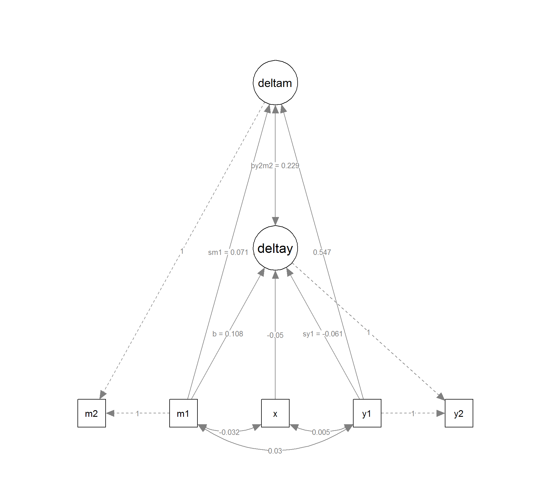
Let’s now inspect a diagram of the model.
# Make new edge labels with path names and unstandardized coefficients
lcs_ancova_ptab <- semPlotModel(lcs_ancova)
lcs_ancova_ptab@Pars$edgeLabels <- ifelse(lcs_ancova_ptab@Pars$label == "",
                          round(lcs_ancova_ptab@Pars$est, digits = 3),
                          sprintf('%s = %.3f', lcs_ancova_ptab@Pars$label, round(lcs_ancova_ptab@Pars$est, digits = 3)))
lcs_ancova_ptab@Pars <- lcs_ancova_ptab@Pars[lcs_ancova_ptab@Pars$edge != "int",]                   # exclude intercepts, we won't be plotting them
lcs_ancova_ptab@Pars <- lcs_ancova_ptab@Pars[lcs_ancova_ptab@Pars$lhs != lcs_ancova_ptab@Pars$rhs,] # exclude residuals, we won't be plotting them

# Plot the LCS ANCOVA mediation model results
semPlot::semPaths(lcs_ancova,
                  edgeLabels = lcs_ancova_ptab@Pars$edgeLabels,
                  layout = "tree",
                  nCharNodes = 0, nCharEdges = 0,
                  what = "path", whatLabels = "path",
                  edge.label.cex = 0.6,
                  residuals = FALSE,                                  # we already excluded residuals
                  intercepts = FALSE,                                 # we already excluded intercepts
                  manifests = c("m2", "m1", "x", "y1", "y2")          # reorder manifest variables to look good
)
References
- Valente, M. J., & MacKinnon, D. P. (2017). Comparing models of change to estimate the mediated effect in the pretest-posttest control group design. Structural equation modeling: a multidisciplinary journal, 24(3), 428-450.
- Valente, M. J., Georgeson, A. R., & Gonzalez, O. (2021). Clarifying the Implicit Assumptions of Two-Wave Mediation Models via the Latent Change Score Specification: An Evaluation of Model Fit Indices. Frontiers in Psychology, 3873.