Exploring Moving Average and other smoothers in R
I. Intro
A smoother is a method for summarizing the trend of a dependent variable as a function of one or more independent variables. It produces an estimate of the trend that is less variable than the dependent variable itself; hence named smoother.
In this short article I will explore simple moving average (SMA), it’s computation, how to plot it and some general information about R functions implementing it. I won’t even mention other types of MA, but will try some point some similarities and differences as it compares to some common, but more sophisticated non-liniar smoothing techniques, like LOESS and cubic splines.
II. Simple Moving Averages
Setup
There are many functions implementing SMA in R. We will load the packages that store them along with some other packages necesary along the road.
Next, for convenience we define our two parameters for SMA. The first is the window the SMA should be computed on, while the second is the offset/alignment.
# Parameters for MA
# Window
window <- 30L

# Offset / Alignment
# With a window of 3:
# align = "right" corresponds to using a window based on offsets of -2, -1, 0, i.e. point before prior, prior and current point. The current point is the rightmost end of the window. Note that rollapplyr with an r on the end is the same as specifying align = "right"
# align = "center" corresponds to using a window based on offsets of -1, 0, 1, i.e. prior point current point and next point. The current point is the center of the window. This is the default for align arguments inside many functions.
# align = "left" corresponds to using a window based on offsets of 0, 1, 2 i.e. current point, next point and point after that. The current point is the leftmost point of the window.
offset <- "right"
Implementing SMA in base R
# Moving average function with base R
# sides = 2 is equivalent to align = "center" for the zoo::rollmean or RcppRoll::roll_mean
# sides = 1 is equivalent to "right" alignment
base_ma <- function(x, n, align = c("right", "center")) {
  align <- match.arg(align)
  if (align == "right") {
    side <- 1
  } else if (align == "center") {
    side <- 2
  }
  as.numeric(stats::filter(x, rep(1 / n, n), sides = side))
}
Using our SMA function we can better understand the offset/alignment parameter.
vec <- 1:10
base_ma(vec, n = 3, align = "right")
## [1] NA NA 2 3 4 5 6 7 8 9
base_ma(vec, n = 3, align = "center")
## [1] NA 2 3 4 5 6 7 8 9 NA
Test SMA on known functions
Here we create two mathematical functions.
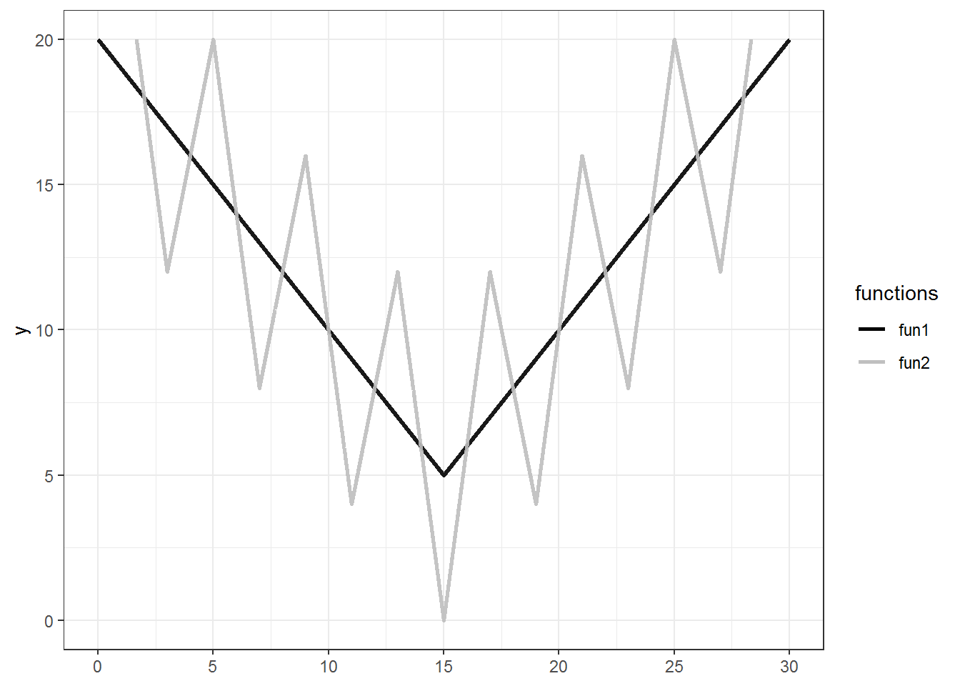
The first function (fun1) is an absolute value function with shift on Ox by c1, Oy by c2 and s scaling parameter controlling how wide the function is.
The second function (fun2) is the summation of the first function with a Triangle wave function.
Both functions being symmetrical, the first may be considered as a possible trend and the second acts like noise that is added to the actual trend (if these where actual data).
This is relevant because centered SMA is considered a technique for detecting trends and identify the turnings points in a trend.
# Absolute value function with shift on Ox by c1, Oy by c2 and s scaling parameter controlling how wide the function is
fun1 <- function(x){c1 = -15; c2 = 5; s = 1; abs(x + c1)*s + c2}   # shift by 15 on Ox, scale it wider by dividing by 2
# Triangle wave function (see https://handwiki.org/wiki/Triangle_wave) with amplitude a and period p
fun_tri <- function(x){a = 5; p = 4; 4*a/p * abs(((x - p/4) %% p) - p/2) - a}
# A composition of the two
fun2 <- function(x){fun1(x) + fun_tri(x)}

plot1 <-
  ggplot() +
  geom_function(fun = fun1, aes(color = "fun1"), size = 1, alpha = 0.9, n = 10^4) +
  geom_function(fun = fun2, aes(color = "fun2"), size = 1, alpha = 0.9, n = 10^4) +
  scale_x_continuous(limits = c(0, 30), breaks = seq(0, 30, by = 5)) +
  scale_y_continuous(limits = c(0, 20), breaks = seq(0, 20, by = 5)) +
  scale_color_manual(name = "functions", values = c("fun1" = "black", "fun2" = "gray")) +
  theme_bw()
## Warning: Using `size` aesthetic for lines was deprecated in ggplot2 3.4.0.
## i Please use `linewidth` instead.
## This warning is displayed once every 8 hours.
## Call `lifecycle::last_lifecycle_warnings()` to see where this warning was
## generated.
plot1
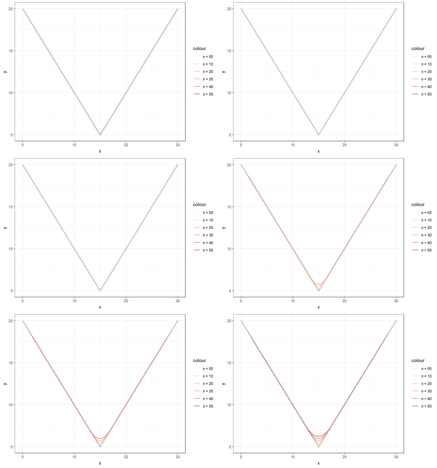
Event with the simple function we can see how the window affects the SMA fit to the data.
data_fun1 <- tibble::tibble(
  x = seq(0, 30, by = .1),
  y = fun1(x),
  ma_fun1_1 = base_ma(y, n = 5, align = "center"),
  ma_fun1_2 = base_ma(y, n = 10, align = "center"),
  ma_fun1_3 = base_ma(y, n = 20, align = "center"),
  ma_fun1_4 = base_ma(y, n = 30, align = "center"),
  ma_fun1_5 = base_ma(y, n = 40, align = "center"),
  ma_fun1_6 = base_ma(y, n = 50, align = "center")
)

ggplot(data_fun1, aes(x = x, y = y)) +
  geom_line(color = "black", size = 1.6, alpha = .2) +
  geom_line(aes(y = ma_fun1_1, color = "n = 05")) +
  geom_line(aes(y = ma_fun1_2, color = "n = 10")) +
  geom_line(aes(y = ma_fun1_3, color = "n = 20")) +
  geom_line(aes(y = ma_fun1_4, color = "n = 30")) +
  geom_line(aes(y = ma_fun1_5, color = "n = 40")) +
  geom_line(aes(y = ma_fun1_6, color = "n = 50")) +
  scale_colour_brewer(palette = "Reds") +
  theme_bw() +
  gganimate::transition_layers(from_blank = FALSE)
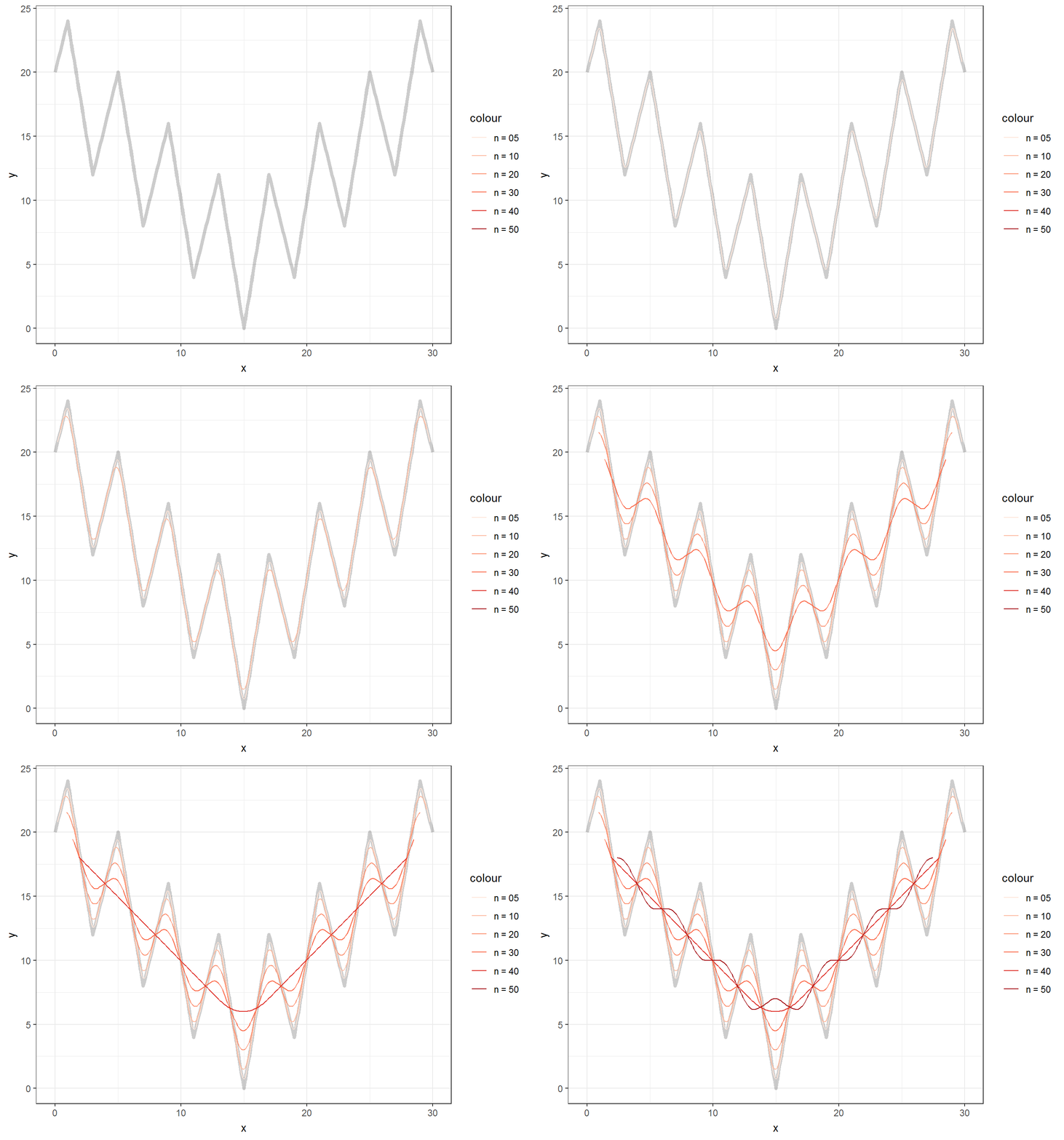
With larger windows, the SMA begins to resemble the trend resembled by the first function (fun1), while the noise of the second function (fun2) is smoothed out of the main picture.
data_fun2 <- tibble::tibble(
  x = seq(0, 30, by = .1),
  y = fun2(x),
  ma_fun2_1 = base_ma(y, n = 5, align = "center"),
  ma_fun2_2 = base_ma(y, n = 10, align = "center"),
  ma_fun2_3 = base_ma(y, n = 20, align = "center"),
  ma_fun2_4 = base_ma(y, n = 30, align = "center"),
  ma_fun2_5 = base_ma(y, n = 40, align = "center"),
  ma_fun2_6 = base_ma(y, n = 50, align = "center")
)

ggplot(data_fun2, aes(x = x, y = y)) +
  geom_line(color = "black", size = 1.6, alpha = .2) +
  geom_line(aes(y = ma_fun2_1, color = "n = 05")) +
  geom_line(aes(y = ma_fun2_2, color = "n = 10")) +
  geom_line(aes(y = ma_fun2_3, color = "n = 20")) +
  geom_line(aes(y = ma_fun2_4, color = "n = 30")) +
  geom_line(aes(y = ma_fun2_5, color = "n = 40")) +
  geom_line(aes(y = ma_fun2_6, color = "n = 50")) +
  scale_colour_brewer(palette = "Reds") +
  theme_bw() +
  gganimate::transition_layers(from_blank = FALSE)
III. SMA in R with actual data
Now that we gathered some intuitions about SMA, let’s get a data set and test what R has to offer in terms of smoothers.
The data
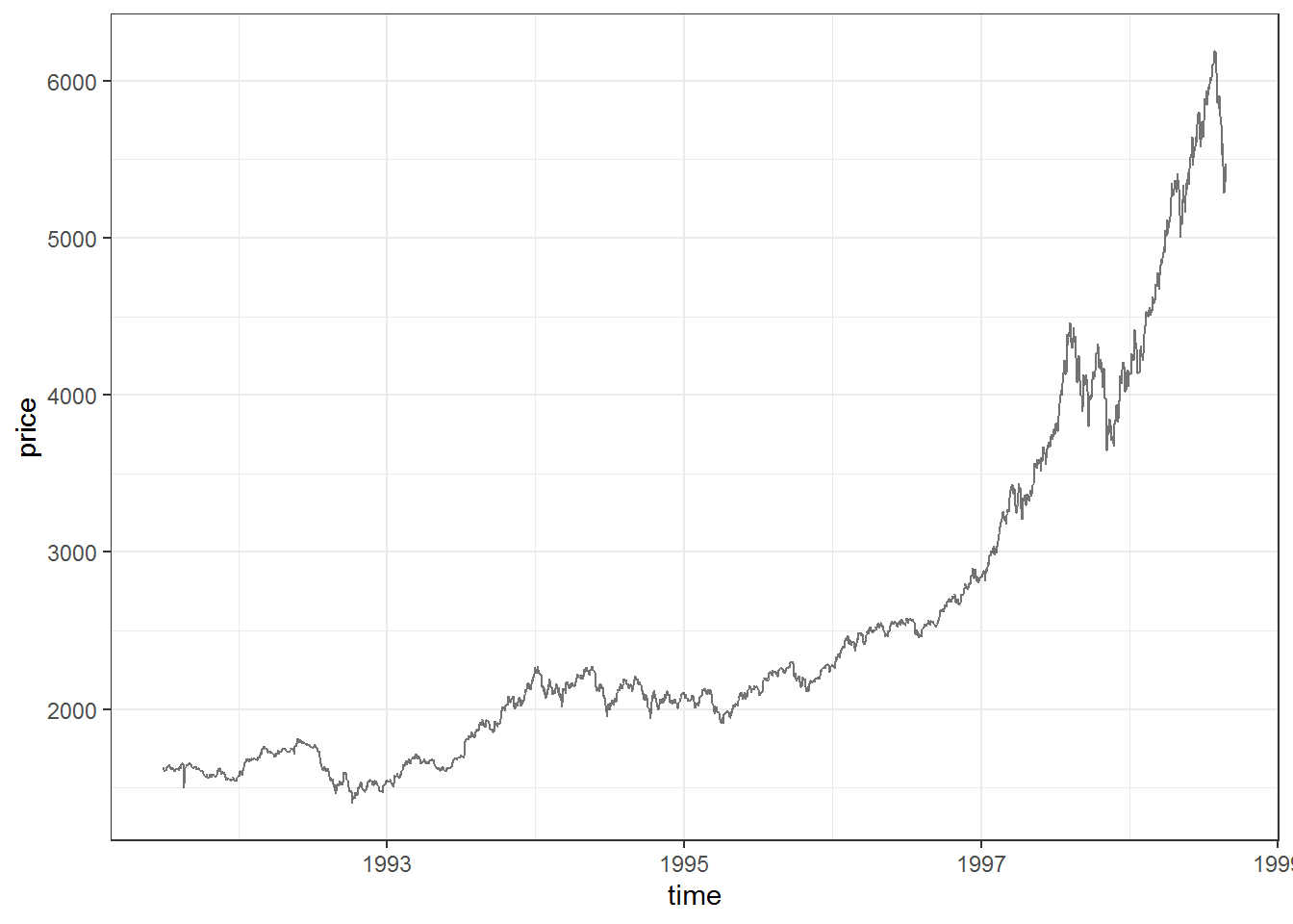
EuStockMarkets data set contains the daily closing prices of major European stock indices, like the Germany DAX (Ibis), for years 1991–1998. Here we will use only the DAX prices.
# Get data
data <-
  datasets::EuStockMarkets %>%
  as.data.frame() %>%
  tidyr::gather(index, price) %>%
  dplyr::mutate(time = rep(time(EuStockMarkets), 4)) %>%
  dplyr::filter(index == "DAX")         # we will use only the DAX data

# Plot the data
plot <- ggplot(data, aes(x = time, y = price)) +
  geom_line(alpha = 0.55, color = "black") +
  theme_bw()

plot
Functions and computation
Functions
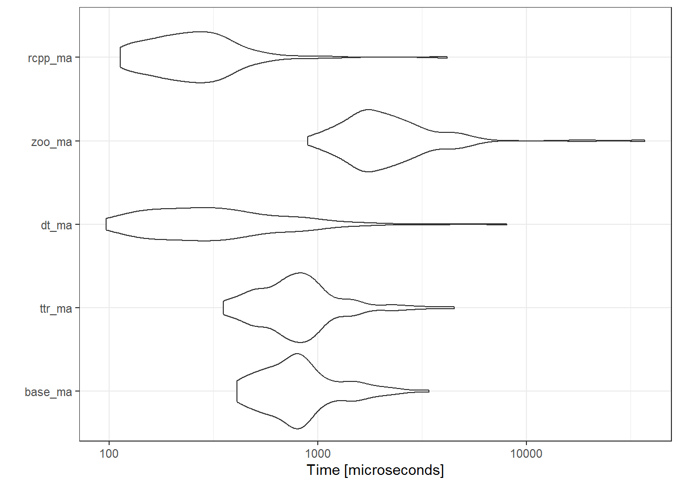
We use our own base R implementation and 4 other very commonly used implementations. The functions in zoo and TTR tend to be used a lot by people in diverse fields interested in time-series, this is probably why these functions constitute the ‘backend’ of many plotting functions for MA. On the other hand, data.table and RcppRoll are very fast, which is not surprising considering both packages are built for speed and minimal external dependencies.
# Compute MA with different functions
data$base_ma <- base_ma(data[, 2], n = window, align = "right")
data$ttr_ma <- TTR::SMA(data[, 2], n = window)    # no possibility of offsetting with an align argument
data$dt_ma <- data.table::frollmean(data[, 2], n = window, align = "right", fill = NA, algo = "fast")
data$zoo_ma <- zoo::rollmean(data[, 2], k = window, align = "right", fill = NA)
data$rcpp_ma <- RcppRoll::roll_mean(data[, 2], n = window, align = "right", fill = NA)
Benchmarking
Clearly, RcppRoll and data.table are the fastest. Our base R function fared decently as well.
# Benchmarking
set.seed(42)
res_bench <-
  microbenchmark::microbenchmark(
    base_ma = base_ma(data[, 2], n = window, align = "right"),
    ttr_ma = TTR::SMA(data[, 2], n = window),
    dt_ma = data.table::frollmean(data[, 2], n = window, align = "right", fill = NA, algo = "fast"),
    zoo_ma = zoo::rollmean(data[, 2], k = window, align = "right", fill = NA),
    rcpp_ma = RcppRoll::roll_mean(data[, 2], n = window, align = "right", fill = NA),
    times = 100L
  )

ggplot2::autoplot(res_bench) +
  theme_bw()
Precision
Precision shouldn’t be such an issue, but if you need very high precision, floating point rounding may affect you. All results seem to be identical (within machine tollerance), except for the function from TTR package.
# Precision
# note that data.table::frollmean() has the `algo` argument set to "fast", while the "exact" algorithm is slower but suffers less from floating point rounding error
all.equal(data$base_ma, data$ttr_ma, tolerance = .Machine$double.eps)
## [1] "Mean relative difference: 8.157587e-16"
all.equal(data$base_ma, data$zoo_ma, tolerance = .Machine$double.eps)
## [1] TRUE
all.equal(data$ttr_ma, data$zoo_ma, tolerance = .Machine$double.eps)
## [1] "Mean relative difference: 8.043689e-16"
all.equal(data$dt_ma, data$zoo_ma, tolerance = .Machine$double.eps)
## [1] TRUE
all.equal(data$dt_ma, data$rcpp_ma, tolerance = .Machine$double.eps)
## [1] TRUE
all.equal(data$rcpp_ma, data$base_ma, tolerance = .Machine$double.eps)
## [1] "Mean relative difference: 2.538355e-16"
Plotting
# Plot
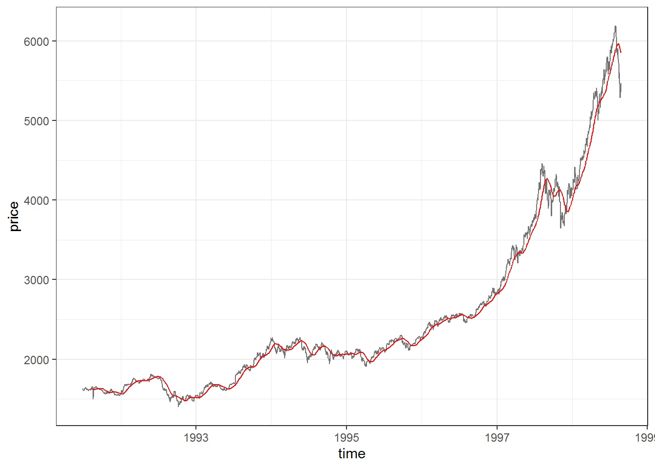
# 1) compute ma and store it in a column inside your data frame
plot +
  geom_line(data = data, aes(y = dt_ma), color = "red")
# 2) compute ma it on the fly
plot +
  geom_line(aes(y = zoo::rollmean(price, k = window, align = "right", na.pad = TRUE)), color = "red")

# 3) compute ma and plot it with tidyquant::geom_ma for ggplot2 (it uses TTR::SMA for simple moving averages)
plot +
  tidyquant::geom_ma(ma_fun = SMA, n = window, color = "red", lty = 1)

IV. SMA and other Smoothers
Loess
Loess, originally named LOWESS (LOcally WEighted Scatter-plot Smoother), is a nonparametric method because of its relaxed linearity assumptions typical of conventional regression methods.
The statsdirect archive lists some important features of the method and its R implementation:
It is called local regression because the fitting at say point x is weighted toward the data nearest to x. The distance from x that is considered near to it is controlled by the span setting,
span.Whenspanis less than 1 it represents the proportion of the data that is considered to be neighbouring x, and the weighting that is used is proportional to 1-(distance/maximum distance)^3)^3, which is known as tricubic. The default span isspan= 0.75. If you choose a span that is too small then there will be insufficient data near x for an accurate fit, resulting in a large variance. If the span is too large than the regression will be over-smoothed, resulting in a loss of information, hence a large bias.
The trade-off between bias and variance also depends on the degree of the polynomial selected. A high degree will provide a better approximation of the population mean, so less bias, but there are more factors to consider in the model, resulting in greater variance. The default degree is 2 (quadratic). Higher degrees don’t improve the fit much. The lower degree (i.e. 1, linear) has more bias but pulls back variance at the boundaries.
plot +
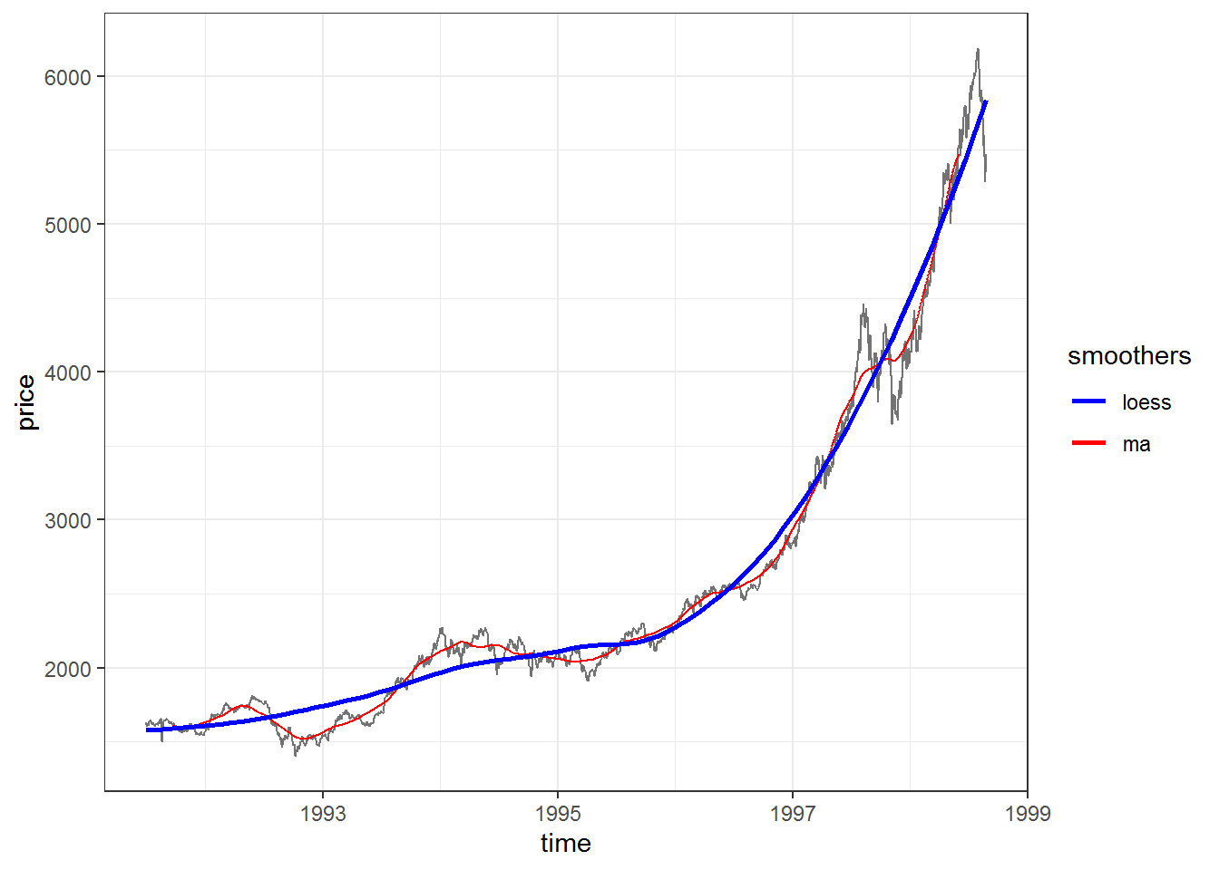
  geom_line(aes(y = zoo::rollmean(price, k = 120, na.pad = TRUE), color = "ma")) +
  geom_smooth(aes(color = "loess"), formula = y ~ x, method = "loess", se = FALSE, span = 0.70) +
  scale_color_manual(name = "smoothers", values = c("ma" = "red", "loess" = "blue"))
Interestingly, using a zero degree polynomial turns LOESS into a weighted moving average
smooth_loess_degree0 <- stats::loess(price ~ time, data = data, span = 0.05, degree = 0)
data$loess_degree0 <- smooth_loess_degree0$fitted

data$ma_largen <- data.table::frollmean(data[, 2], n = 55, align = "center", fill = NA, algo = "fast")

plot +
  geom_line(data = data, aes(y = ma_largen, color = "ma"), size = 0.5) +
  geom_line(data = data, aes(y = loess_degree0, color = "loess"), size = 0.5) +
  scale_color_manual(name = "smoothers", values = c("ma" = "red", "loess" = "blue"))
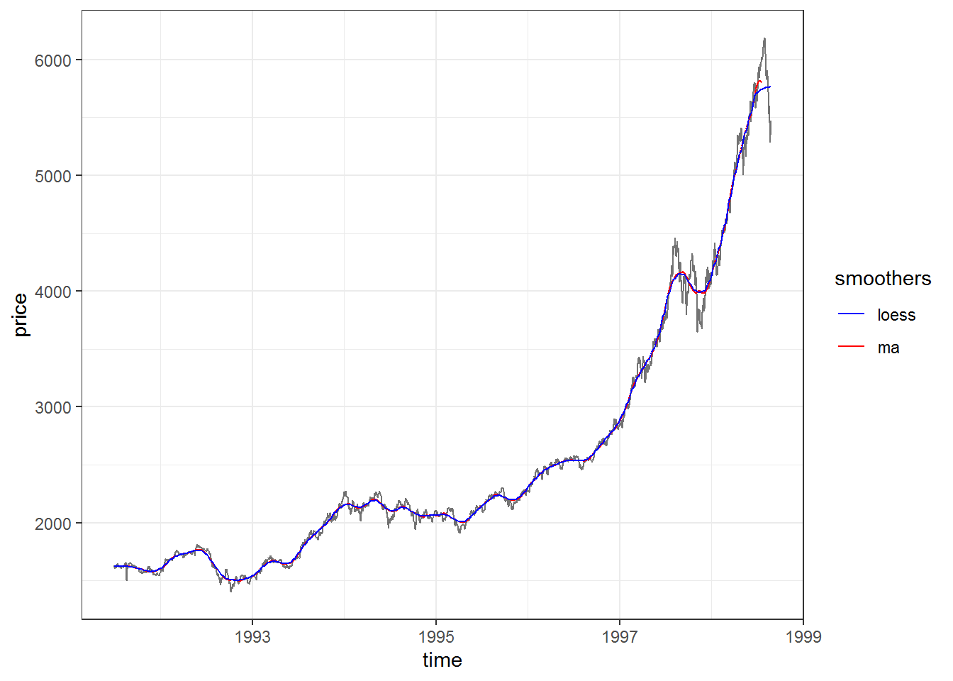
It is however important to note that Loess is non-liniar (unlike local regression and liniar splines) and proposes a degree of “robustification” to outliers (by downweighting large residuals and refitting). As a result, in the general case, Loess results won’t be exactly reproduced by liniar methods.
Generalized Additive model with Penalized Cubic regression splines
A cubic spline smoother is a solution to the following optimization problem: among all smooth unknown functions with second continuous derivatives, find one that minimizes the penalized least square.
The name cubic spline is from the piecewise polynomial fit, with order = 3, where most study shown that order = 3 is sufficient.
gamma is a non-negative smoothing parameter that must be chosen by the data analyst. It governs the tradeoff between the goodness of fit to the data and the wiggleness of the function. It plays nearly the same role as span (the percentage of data points used as nearest neighbors in percent of total n) in other smoothing methods, like Loess.
Here I will try to tweak the Generalized Additive model with Penalized Cubic regression splines in order to produce results similar to SMA.
library(mgcv)

smooth_gam_cubspline <- mgcv::gam(price ~ s(time, k = 50, bs = "cs"), data = data, method = "REML", gamma = 4)
data$gam_cubspline <- smooth_gam_cubspline$fitted.values

plot +
  geom_line(data = data, aes(y = ma_largen, color = "ma"), size = 0.5) +
  geom_line(data = data, aes(y = gam_cubspline, color = "cubic splines"), size = 0.5) +
  scale_color_manual(name = "smoothers", values = c("ma" = "red", "cubic splines" = "green"))
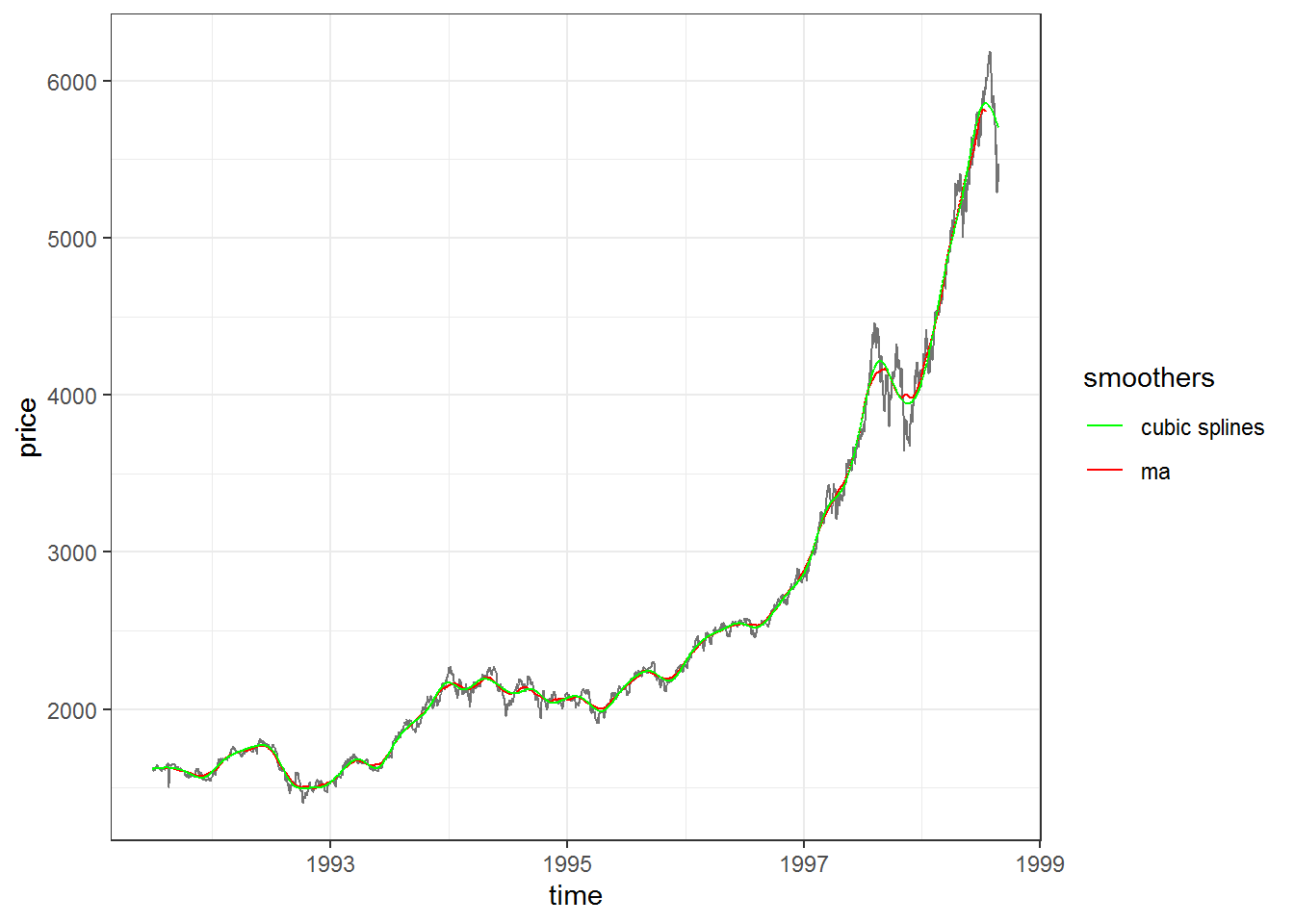
Again, by tweeking the parameters, we see that Loess and GAM with penalized cubic splines give very very close results to SMA.
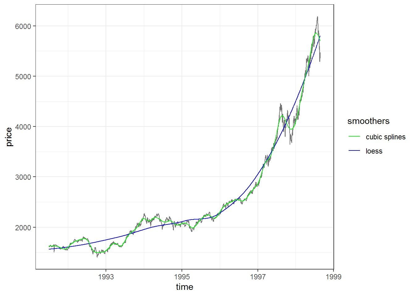
Although Loess and GAM with cubic splines are very different methods, they are the most used adaptive smoothers and are frequently used interchangeably whenever someone needs to glance at the trend in some data. In fact, ggplot2::geom_smooth() actually switches its default smooth method from Loess to a Generalized Additive Model with Penilized Cubic splines once n is > 1000 (it does this as Loess is O(n²) in memory so it might be slow on large data).
The last caveat is that our tweaking to make these smoothers give similar results to SMA does not do them justice. This is why the last subchapter is dedicated to their results on default settings.
Loess vs Cubic splines
data$loess <- stats::loess(price ~ time, data = data)$fitted
data$gam <- mgcv::gam(price ~ s(time, bs = "cs"), data = data, method = "REML")$fitted.values

plot +
  geom_line(data = data, aes(y = loess, color = "loess"), size = 0.5) +
  geom_line(data = data, aes(y = gam_cubspline, color = "cubic splines"), size = 0.5) +
  scale_color_manual(name = "smoothers", values = c("loess" = "blue", "cubic splines" = "green"))
