Automated systematic literature search using R, litsearchr, and Google Scholar web scraping
Introduction
You would like to do a systematic search of the scientific literature on a given topic. But a wild caveat appears - your familiarity (or lack there of) with the topic will bias your search, while your field lacks in standardized terminology and is fragmented into multiple nomenclature clusters.
Grames et al. (2019) devised a method to address this (you can read the article here). A gentle introduction to both R and litsearchr package that trivializes the analyses can be found on Library Carpentry.
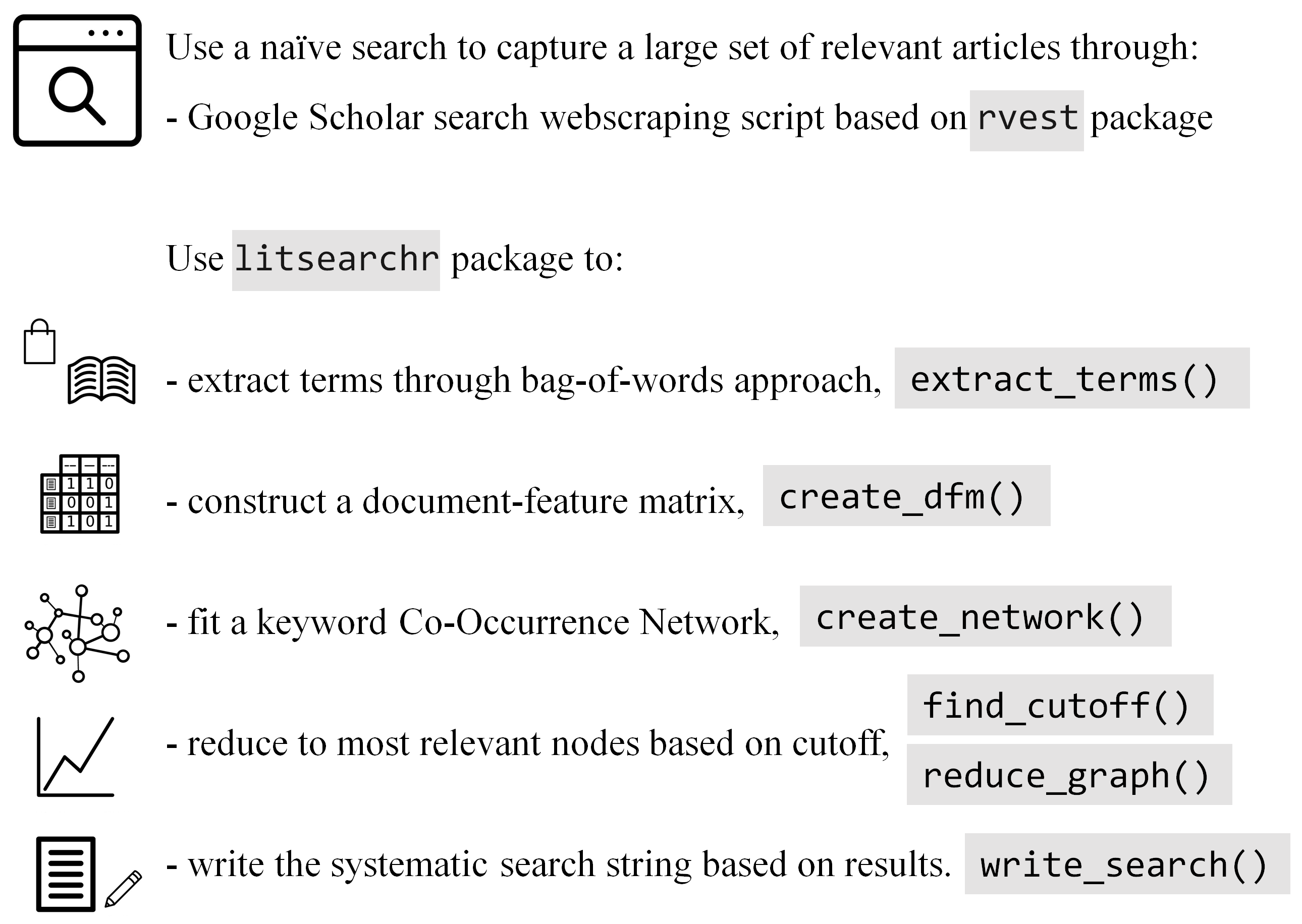
Simply put we can cast a wide net using a naïve search, retrieve relevant information from data bases (e.g., titles, keywords, abstracts) and analyse this interlinked text data to derive a systematic search strategy. I view it as way to bootstrap knowledge.

This is a followup on a previous post that presents the same same procedure but using PubMed API curtsy of easyPubMed package. Unfortunately, Google Scholar has no API, so here will just scrape titles and sections of abstracts. Keep in mind that scraping Google Scholar is not polite, that the process take a long time due to rate limiting and that using only expressions from article titles is generally less effective than using multiple sources together (e.g. titles, keywords, and possibly full abstracts).
We will use:
- my Scholar Google search web scraping function to extract literature metadata based on an preliminary naïve search query.
easyPubMedthat simplifies the use of the PubMed API to query and extract article data.litsearchrfor automated approach to identifying search terms for systematic reviews using keyword co-occurrence networks.stopwordsfor the Stopwords ISO Dataset which is the most comprehensive collection of stopwords for multiple languages.igraphfor network analyses (this package is already a dependence oflitsearchrbut there are still many useful functions that are not wrapped bylitsearchrfunctions).ggplot2,ggraph, andggrepelfor plotting.
1. Load or install packages
# litsearchr isn't yet on CRAN, need to install from github
if (require(litsearchr)) remotes::install_github("elizagrames/litsearchr", ref = "main")

# Packages to load/install
packages <- c(
  "easyPubMed",
  "litsearchr", "stopwords", "igraph",
  "ggplot2", "ggraph", "ggrepel"
)

# Install packages not yet installed
installed_packages <- packages %in% rownames(installed.packages())
if (any(installed_packages == FALSE)) {
  install.packages(packages[!installed_packages])
}

# Load packages
lapply(packages, library, character.only = TRUE)
2. Run the web scraping function
# Source web scraping function
devtools::source_gist("https://gist.github.com/ClaudiuPapasteri/7bef34394c395e03ee074f884ddbf4d4")
If you use proxies you should check that they are working:
########################
if (require(jsonlite)) install.packages("jsonlite")
library(jsonlite)

# get your IP
jsonlite::fromJSON(rvest::html_text(rvest::read_html("http://jsonip.com/")))$ip

# test proxy
session <- rvest::session("http://jsonip.com/",
                          httr::user_agent("Mozilla/5.0 (Windows NT 10.0; Win64; x64) AppleWebKit/537.36 (KHTML, like Gecko) Chrome/58.0.3029.110 Safari/537.36"),
                          httr::use_proxy(url = "XXXX", port = 8888,
                                          username = "XXXX", password = "XXXX"))
page_text <- rvest::html_text(rvest::read_html(session))
proxy_ip <- jsonlite::fromJSON(page_text)$ip
proxy_ip
#####################
# Scrape Scholar Google
useragent <- httr::user_agent("Mozilla/5.0 (Windows NT 10.0; Win64; x64) AppleWebKit/537.36 (KHTML, like Gecko) Chrome/110.0.0.0 Safari/537.36")
# proxy1 <- httr::use_proxy("5.78.83.190", port = 8080)  # can pass proxy to function; here we just scrape patiently and don't use proxy
gs_df1 <- scrape_gs(term = 'intext:"psychotherapy" AND "PTSD"', pages = 1:20, crawl_delay = 1.2, useragent)  # scrape first 20 pages (200 published works)
# even with some human-like behavior, the crawling script still gets blocked by server if run too long
gs_df2 <- scrape_gs(term = 'intext:"psychotherapy" AND "PTSD"', pages = 21:40, crawl_delay = 1.2, useragent)  # scrape next 20 pages (200 published works)
# if you don't have proxies, just scrape sequentially and cache results
gs_df3 <- scrape_gs(term = 'intext:"psychotherapy" AND "PTSD"', pages = 41:60, crawl_delay = 1.2, useragent)  # scrape next 20 pages (200 published works)
# if you don't have proxies, just scrape sequentially and cache results
gs_df4 <- scrape_gs(term = 'intext:"psychotherapy" AND "PTSD"', pages = 61:80, crawl_delay = 1.2, useragent)  # scrape next 20 pages (200 published works)
# we stopped at page 99 because that's how many pages Google Scholar gives us
gs_df5 <- scrape_gs(term = 'intext:"psychotherapy" AND "PTSD"', pages = 81:99, crawl_delay = 1.2, useragent)  # scrape last 19 pages (190 published works)
Check the first 10 entries:
gs_df <- rbind(gs_df1, gs_df2, gs_df3, gs_df4, gs_df5)  # total of 99 pages (990 published works)

# See results
head(gs_df)
##   page                              term
## 1    1 intext:"psychotherapy" AND "PTSD"
## 2    1 intext:"psychotherapy" AND "PTSD"
## 3    1 intext:"psychotherapy" AND "PTSD"
## 4    1 intext:"psychotherapy" AND "PTSD"
## 5    1 intext:"psychotherapy" AND "PTSD"
## 6    1 intext:"psychotherapy" AND "PTSD"
##                                                                                                                     title
## 1                                                              A multidimensional meta-analysis of psychotherapy for PTSD
## 2                              Inclusion and exclusion criteria in randomized controlled trials of psychotherapy for PTSD
## 3                                                                     A guide to the literature on psychotherapy for PTSD
## 4                              Is exposure necessary? A randomized clinical trial of interpersonal psychotherapy for PTSD
## 5                                                 Changes in cortisol and DHEA plasma levels after psychotherapy for PTSD
## 6 Factors associated with completing evidence-based psychotherapy for PTSD among veterans in a national healthcare system
##                                        authors year n_citations
## 1         R Bradley, J Greene, E Russ, L Dutra 2005        2675
## 2               JM Ronconi, B Shiner, BV Watts 2014          99
## 3          JL Hamblen, PP Schnurr, A Rosenberg 2009          42
## 4             JC Markowitz, E Petkova, Y Neria 2015         367
## 5    M Olff, GJ de Vries, Y Güzelcan, J Assies 2007         217
## 6 S Maguen, Y Li, E Madden, KH Seal, TC Neylan 2019          79
##                                                                                                                                                                                        abstract
## 1         … 1980 and 2003 on psychotherapy for PTSD. METHOD: Data on … RESULTS: Results suggest \nthat psychotherapy for PTSD … of patients treated with psychotherapy for PTSD in randomized …
## 2     … , our study suggests that psychotherapy for PTSD has likely been … psychotherapy for PTSD \nwould appear to be applicable to clinical populations. Patients with the most common PTSD …
## 3       … nonspecific benefits of psychotherapy. Both groups had a modest decrease in PTSD symptoms, \nbut contrary to expectations, CBT was not more effective than present-centered therapy.…
## 4    … in psychotherapy for posttraumatic stress disorder (PTSD). The authors tested \ninterpersonal psychotherapy (… in pilot PTSD research as a non-exposure-based non-cognitive-behavioral …
## 5 … psychotherapy the low basal cortisol levels in PTSD patients would increase. To our knowledge \nthis is the first study to assess the effects of psychotherapy in PTSD on these hormones. …
## 6      … of Iraq and Afghanistan veterans with PTSD. PTSD visits were linked to 8.1 million psychotherapy \nnotes, and annotators labeled 3467 randomly-selected psychotherapy notes (kappa = …
Note that I ran this for several days to scrape each chunk of 20 pages. If you scrape continuously, the server will either respond with HTTP Error 429: Too Many Requests or with a Captcha page. If you run into issues and no informative error message is displayed, check if ran into a Captcha page:
gs_url_base <- "https://scholar.google.com/scholar"
term <- 'intext:"psychotherapy" AND "PTSD"'
page_no <- 90
gs_url <- paste0(gs_url_base, "?start=", page_no - 1, "&q=", noquote(gsub("\\s+", "+", trimws(term))))
session <- rvest::session(gs_url)
wbpage <- rvest::read_html(session)
page_text <- rvest::html_text(wbpage)
page_text  # check what the page displays
captcha <- rvest::html_text(rvest::html_elements(wbpage, "#gs_captcha_ccl"))
captcha   # check if there is a captcha
3. Extract terms from scraped data
To extract interesting words out of titles use the Rapid Automatic Keyword Extraction (RAKE) algorithm, coupled with a good stop word collection.
# Extract terms from from title
gs_terms <- litsearchr::extract_terms(text = gs_df[,"title"],
                                      method = "fakerake", min_freq = 3, min_n = 2,
                                      stopwords = stopwords::data_stopwords_stopwordsiso$en)
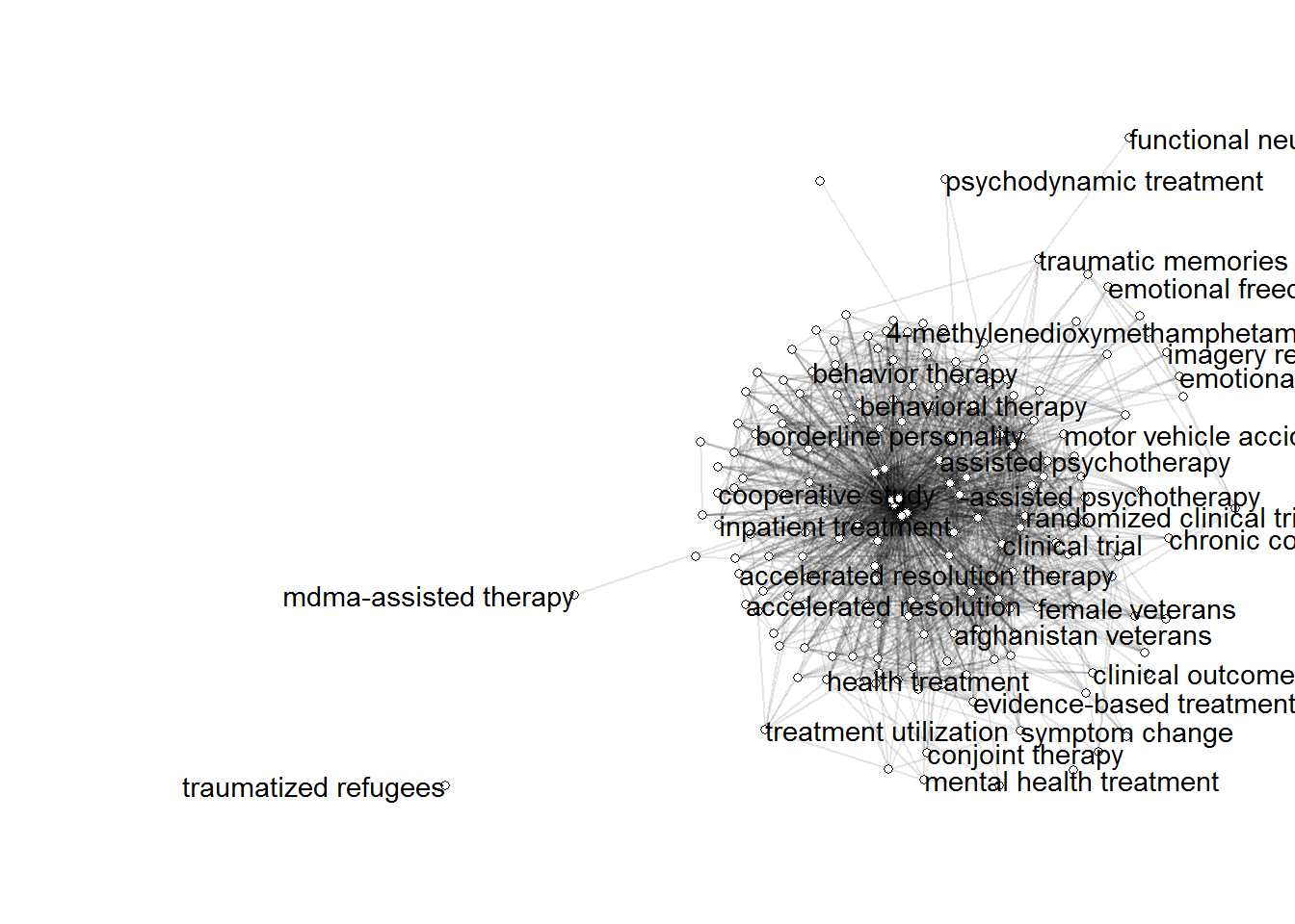
4. Create Co-Occurrence Network
We will consider the title and abstract of each article to represent the article’s “content” and we will consider a term to have appeared in the article if it appears in either the title or abstract. Based on this we will create the document-feature matrix, where the “documents” are our articles (title and abstract) and the “features” are the search terms. The Co-Occurrence Network is computed using this document-feature matrix.
# Create Co-Occurrence Network
gs_docs <- paste(gs_df[, "title"], gs_df[, "abstract"]) # we will consider title and abstract of each article to represent the article's "content"
gs_dfm <- litsearchr::create_dfm(elements = gs_docs, features = gs_terms) # document-feature matrix
gs_coocnet <- litsearchr::create_network(gs_dfm, min_studies = 3)

ggraph(gs_coocnet, layout = "stress") +
  coord_fixed() +
  expand_limits(x = c(-3, 3)) +
  geom_edge_link(aes(alpha = weight)) +
  geom_node_point(shape = "circle filled", fill = "white") +
  geom_node_text(aes(label = name), hjust = "outward", check_overlap = TRUE) +
  guides(edge_alpha = "none") +
  theme_void()

5. Prune the Network based on node strength
5.1 Compute node strength
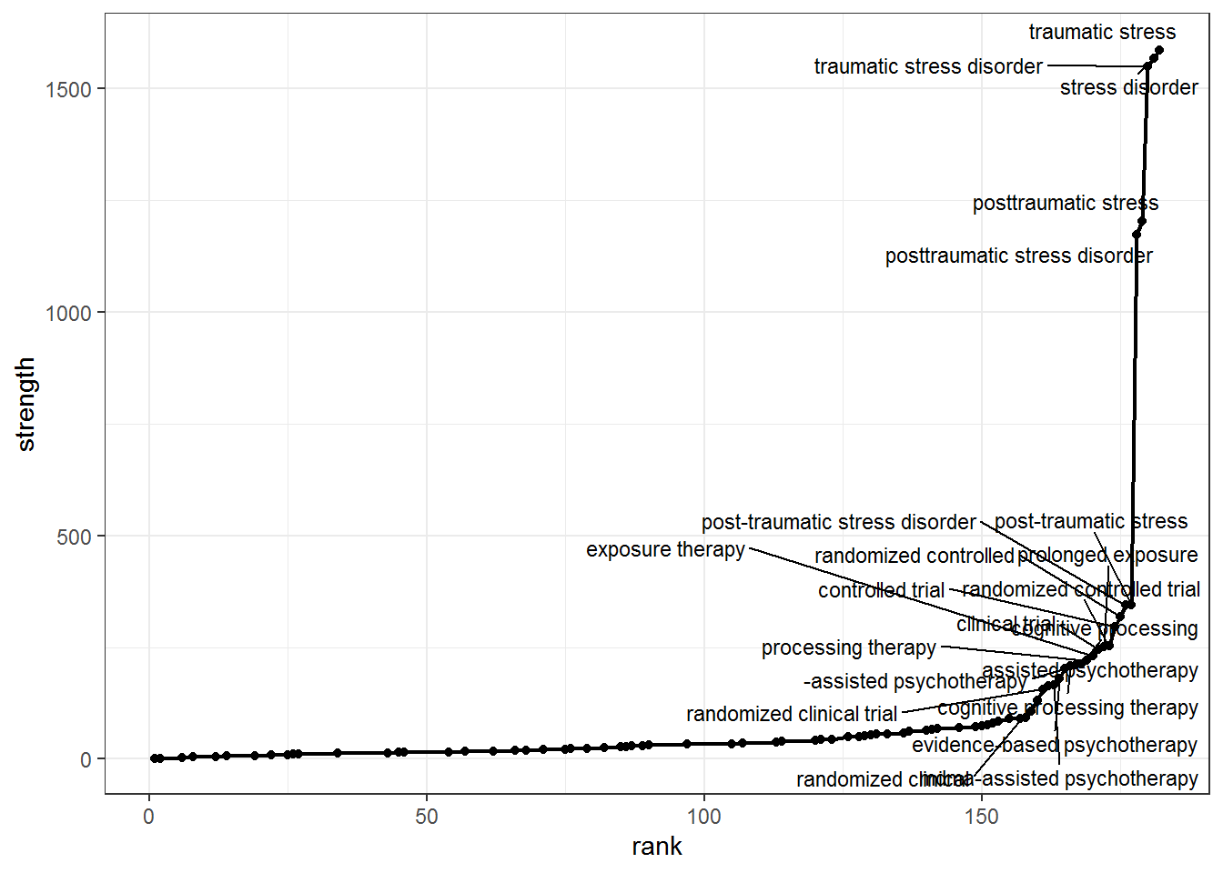
Node strength in a network is calculated by summing up the weights of all edges connected to the respective node.Thus, node strength investigates how strongly it is directly connected to other nodes in the network.
# Prune the Network based on node strength
gs_node_strength <- igraph::strength(gs_coocnet)
gs_node_rankstrenght <- data.frame(term = names(gs_node_strength), strength = gs_node_strength, row.names = NULL)
gs_node_rankstrenght$rank <- rank(gs_node_rankstrenght$strength, ties.method = "min")
gs_node_rankstrenght <- gs_node_rankstrenght[order(gs_node_rankstrenght$rank),]

gs_plot_strenght <-
  ggplot(gs_node_rankstrenght, aes(x = rank, y = strength, label = term)) +
  geom_line(lwd = 0.8) +
  geom_point() +
  ggrepel::geom_text_repel(size = 3, hjust = "right", nudge_y = 3, max.overlaps = 30) +
  theme_bw()
gs_plot_strenght

5.1 Prune based on chosen criteria
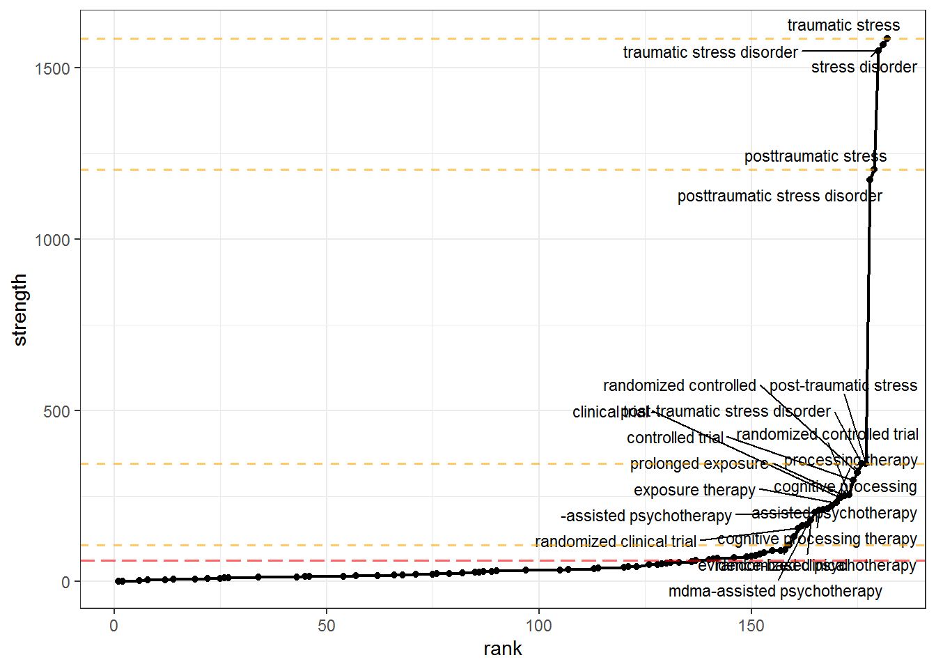
We want to keep only those nodes that have high strength, but how will we decide how many to prune out? litsearchr::find_cutoff() provides us with two ways to decide: cumulative cutoff and change points. The cumulative cutoff method simply retains a certain proportion of the total strength. The change points method uses changepoint::cpt.mean() under the hood to calculate optimal cutoff positions where the trend in strength shows sharp changes.
Again, we will use the heuristic when in doubt, pool results together, i.e. we will use the change point nearest the to the cumulative cutoff value we set.
# Cumulatively - retain a certain proportion (e.g. 80%) of the total strength of the network of search terms
gs_cutoff_cum <- litsearchr::find_cutoff(gs_coocnet, method = "cumulative", percent = 0.8)
# Changepoints - certain points along the ranking of terms where the strength of the next strongest term is much greater than that of the previous one
gs_cutoff_change <- litsearchr::find_cutoff(gs_coocnet, method = "changepoint", knot_num = 3)

gs_plot_strenght +
  geom_hline(yintercept = gs_cutoff_cum, color = "red", lwd = 0.7, linetype = "longdash", alpha = 0.6) +
  geom_hline(yintercept = gs_cutoff_change, color = "orange", lwd = 0.7, linetype = "dashed", alpha = 0.6)

gs_cutoff_crit <- gs_cutoff_change[which.min(abs(gs_cutoff_change - gs_cutoff_cum))]  # e.g. nearest cutpoint to cumulative criterion (cumulative produces one value, changepoints may be many)

gs_maxselected_terms <- litsearchr::get_keywords(litsearchr::reduce_graph(gs_coocnet, gs_cutoff_crit))
Inspect selected terms:
gs_maxselected_terms
##  [1] "-assisted psychotherapy"        "assisted psychotherapy"
##  [3] "clinical trial"                 "cognitive processing"
##  [5] "cognitive processing therapy"   "controlled trial"
##  [7] "evidence-based psychotherapy"   "exposure therapy"
##  [9] "mdma-assisted psychotherapy"    "post-traumatic stress"
## [11] "post-traumatic stress disorder" "posttraumatic stress"
## [13] "posttraumatic stress disorder"  "processing therapy"
## [15] "prolonged exposure"             "prolonged exposure therapy"
## [17] "randomized clinical"            "randomized clinical trial"
## [19] "randomized controlled"          "randomized controlled trial"
## [21] "stress disorder"                "systematic review"
## [23] "traumatic stress"               "traumatic stress disorder"
Some expression already contain others. For example, “mdma-assisted psychotherapy” is an instance of “-assisted psychotherapy” which is a very important key term that defines psychotherapies that use pharmacological means or other tools to achieve it’s results. This happens for a lot of strings, and generally, we would like to keep only the shortest unique substring
Keep only shortest unique substrings:
superstring <- rep(FALSE, length(gs_maxselected_terms))
for(i in seq_len(length(gs_maxselected_terms))) {
  superstring[i] <- any(stringr::str_detect(gs_maxselected_terms[i], gs_maxselected_terms[-which(gs_maxselected_terms == gs_maxselected_terms[i])]))
}
gs_selected_terms <- gs_maxselected_terms[!superstring]
We will also manually do two other changes: (1) we are not interested in “systematic reviews” so we will remove it; (2) we will add the terms “psychotherapy” and “ptsd” as they are not already present in their simplest form.
gs_selected_terms <- gs_selected_terms[-which(gs_selected_terms == "systematic review")]
gs_selected_terms <- c(gs_selected_terms, "psychotherapy", "ptsd")
Inspect selected terms:
gs_selected_terms
##  [1] "assisted psychotherapy"       "clinical trial"
##  [3] "cognitive processing"         "controlled trial"
##  [5] "evidence-based psychotherapy" "exposure therapy"
##  [7] "processing therapy"           "prolonged exposure"
##  [9] "randomized clinical"          "randomized controlled"
## [11] "stress disorder"              "traumatic stress"
## [13] "psychotherapy"                "ptsd"
We see that term groupings are obvious: type of study (design), type of intervention, disorder/symptoms, and population.
6. Manual grouping into clusters
# Manual grouping into clusters - for more rigorous search we will need a combination of OR and AND operators
design <- gs_selected_terms[c(2, 4, 9, 10)]
intervention <- gs_selected_terms[c(1, 3, 5, 6, 7, 8, 13)]
disorder <- gs_selected_terms[c(11, 12, 14)]

# all.equal(length(gs_selected_terms),
#   sum(length(design), length(intervention), length(disorder))
# )  # check that we grouped all terms

gs_gruped_selected_terms <- list(
  design = design,
  intervention = intervention,
  disorder = disorder
)
7. Automatically write the search string
# Write the search
litsearchr::write_search(
  gs_gruped_selected_terms,
  languages = "English",
  exactphrase = TRUE,
  stemming = FALSE,
  closure = "left",
  writesearch = FALSE
)
## [1] "English is written"
## [1] "((\"clinical trial\" OR \"controlled trial\" OR \"randomized clinical\" OR \"randomized controlled\") AND (\"assisted psychotherapy\" OR \"cognitive processing\" OR \"evidence-based psychotherapy\" OR \"exposure therapy\" OR \"processing therapy\" OR \"prolonged exposure\" OR psychotherapy) AND (\"stress disorder\" OR \"traumatic stress\" OR ptsd))"
Discussions
Only the last two steps, pertaining to term exclusion and term grouping, need the careful decisions of a human researcher. The automatic workflow, on it’s own, found some important terms that I would have surely omitted. I am especially pleased about “exposure therapy”, “cognitive processing”, “processing therapy” which describe classes of psychotherapy interventions but lack the prefix “psycho-”, making it harder to distinguish them from other non-psychotherapy interventions simply termed “therapy”. Also, the method correctly identifies “assisted psychotherapy” where pharmacological agents are used, which is another important niche that may be easily omitted.
References
Grames, E. M., Stillman, A. N., Tingley, M. W., & Elphick, C. S. (2019). An automated approach to identifying search terms for systematic reviews using keyword co‐occurrence networks. Methods in Ecology and Evolution, 10(10), 1645-1654.